Software

Kotlin, command-based, simulated first.

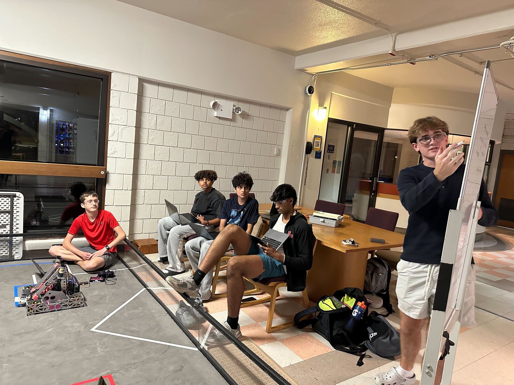
We rewrote our Java code in Kotlin so several of us can work at once, and every change goes through a reviewed pull request.

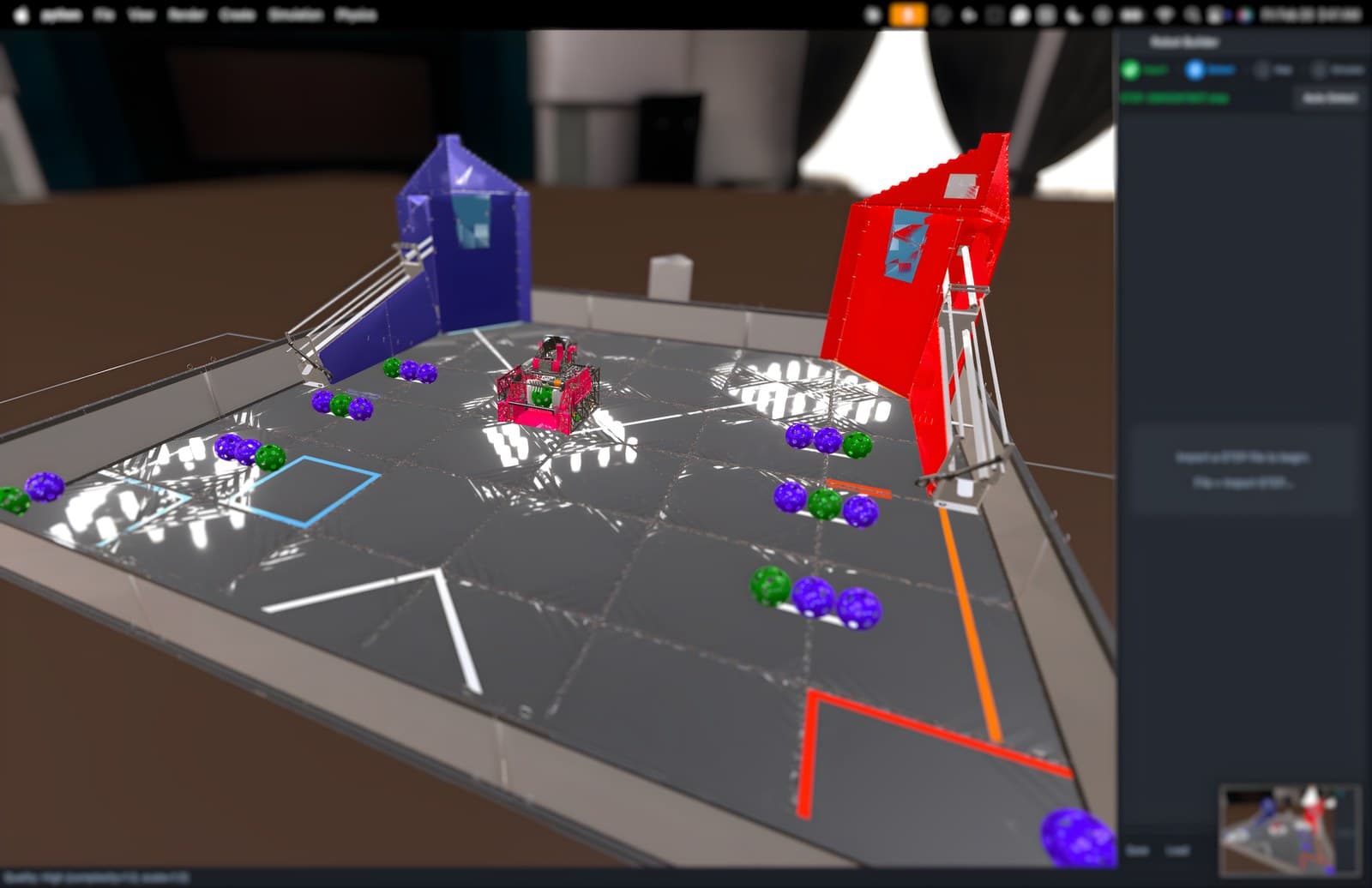
The simulated robot on the field in our USD viewport

Simulation

The same code runs on the robot and in simulation

We abstracted the robot's inputs and outputs so one codebase runs on hardware and in a simulator. The simulator runs as a unit test with no Android dependencies, and you can drive it with a normal game controller.

It renders in real time in a USD viewport, with CAD imported straight from STEP files. That's how drivers practise when the robot is in pieces on the bench.

Details

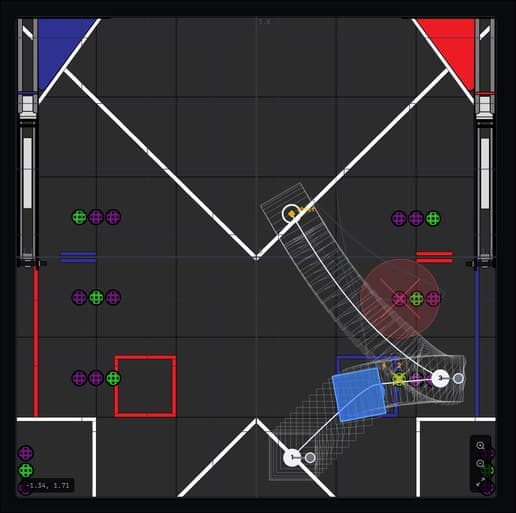
A second simulator runs in the browser on the Jolt physics engine and Three.js. We use it to check autonomous paths.

Both use a physics model that combines motor dynamics, mecanum kinematics and projectile motion, so we can find the robot's limits before testing on hardware.
State machine: one button press moves from idle to intake, index and shoot, then back to idleIdleIntakeIndexShootone button

Driver automation

One button runs the whole cycle

A finite state machine runs the multi-step sequences: intake, index, shoot. Kotlin's async functions run hardware tasks at the same time and wait for them to finish before moving on.

The driver presses one button for a full cycle instead of juggling four inputs mid-match.

Details

Because each state waits for its hardware tasks to finish before the next one starts, the sequence holds together when a mechanism runs slow.

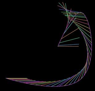
Optimised path drawn across the field in our path editor

Path optimisation

We plan the fastest path, and built our own editor

We set up each trajectory between waypoints as an optimisation problem, with modelled motor limits and shortest travel time as the goal.

Inspired by FRC's Choreo, we built a web editor for these paths, so tuning an autonomous doesn't mean editing numbers in source code.

Details

PedroPathing handles the autonomous trajectories on the robot.

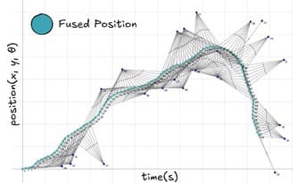
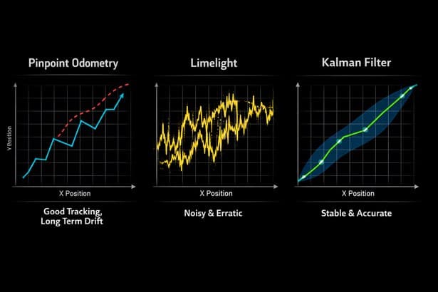
Plot of odometry and vision estimates merged by the Kalman filter

Localization

Odometry and vision, corrected as the robot moves

In TeleOp a Kalman filter fuses Pinpoint odometry with Limelight vision. It weights each sensor by how much to trust it, so noisy vision readings get rejected but real corrections still land.

On the Worlds robot a factor graph does the same job with AprilTag sightings.

Details

The Limelight reads AprilTags for position and the motif pattern, and runs our own artifact classifier on its coprocessor.

We label training data with Meta's Segment Anything Model and train the competition model on Duke University's H200 GPU cluster.

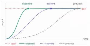
Chart comparing measured control performance against the goal over time

Control

We model the robot, then control it against the model

For the Worlds robot we modelled its motion and mechanisms, then used those models for planning and feedback control.

Every control loop gets measured on each change against its previous and expected performance. That's what makes it safe to keep rewriting the control code mid-season.

Details

A global shutter camera and an OAK stereo camera watch real shots, so the shooter maps flywheel RPM and hood angle to arcs it actually observed.

Optimal control

Writing the fastest path as a problem a solver can answer

This is how a time-optimal trajectory can be written. It's an illustration, not the exact solver on the robot.

min⁡N, u0,…,uN−1NΔtsubject toN∈Z>0,xk+1=f(xk,uk),k=0,…,N−1,x0=xstart,xN∈Xgoal,xk∈X,uk∈U\begin{aligned} \min_{N,\,u_0,\ldots,u_{N-1}}\quad & N\Delta t \\ \text{subject to}\quad & N\in\mathbb{Z}_{>0},\\ & x_{k+1}=f(x_k,u_k), \quad k=0,\ldots,N-1,\\ & x_0=x_{\mathrm{start}}, \quad x_N\in\mathcal{X}_{\mathrm{goal}},\\ & x_k\in\mathcal{X}, \quad u_k\in\mathcal{U} \end{aligned}
N is the number of control steps and Δt is the length of each step in seconds. At each step, x is the robot state, u is the motor command and f is the motion model. X and U are the modelled state and command limits, and the goal set holds the acceptable final poses and speeds.
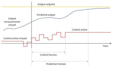
Model Predictive Control plot

Model-based trajectory planning

Model Predictive Control

Uses a robot model to evaluate future motion and choose control inputs within modeled drivetrain limits. The trajectory objective favors shorter traversal time; the result depends on model accuracy and the chosen constraints.

Factor-graph localization plot

Corrects accumulated odometry drift

Factor-graph localization

A GTSAM factor graph combines odometry with Limelight AprilTag observations to update the robot's pose. Reliable tag observations can correct error accumulated by odometry.

LTV path following plot

Feedback along a reference path

LTV path following

We linearize the motion model around a reference path and use a Linear Time-Varying controller to update drive commands as the robot moves. Performance depends on how closely the model and reference match the robot's motion.

From the code

How the shooter picks its speed

A trimmed excerpt from Shooter.kt in last season's robot code. Distance to the goal sets the target RPM from a curve we fitted to test shots, and the hood corrects for any RPM error.

Shooter.kt · 2025-Decode
// Shooter RPM = 102.14973x^2 + 81.22682x + 2739.19625 (x is distance from goal in meters)val actualRPM = hardware.shooterRPM() * Constants.ShooterConstants.gearRatio val output = pidController.calculate(actualRPM, if (isRunning) { targetRPM } else if (idleMode) { Constants.ShooterConstants.idleRPM } else { 0.0 }).coerceIn(-1.0, 1.0) // less than 3% RPM ErrorisUpToSpeed = (actualRPM - targetRPM).absoluteValue / targetRPM > 0.03 if (!idleMode) {    // adjust hood based on shooter testing data    val rpmDifference = actualRPM - targetRPM    val hoodOffset = rpmDifference * -0.0004    hardware.hood = (targetHood + hoodOffset).clamp(        Constants.ShooterConstants.hoodFullUp,        Constants.ShooterConstants.hoodFullDown    )}

How we write code

Git for version control with conventional commits, so the history reads cleanly. Every pull request needs at least two human reviewers before it merges. We use agentic AI to accelerate development, but we architect the key systems and write the hard parts ourselves.

How we use AI

We use AI for repetitive code that needs little critical thinking. Every AI-written line is reviewed by the programmer who prompted it, then again in a PR review — two cycles of human review. Advanced systems have their architecture planned before AI touches them.